5 Advanced access to the database
Connecting to and working with the database as described in the last section is rather easy, but this comes at a price - very limited possibilities. The front-end “DB Admin” is much more powerful, but you have to have a basic understanding about how databases work in general as well as some understanding of the particular database implementation. Therefore this section continues with an introduction on the database basics, but first you have to connect to the database:
Open http://woodcar.boku.ac.at/ in your web-browser and click on the link for “DB Admin” to open the login page. You could use the front-end to connect to any database, therefore you need to provide all necessary information:
- System: Select the database driver - for PostgreSQL in our case
- Server: the path to the database-server:
dazzling-calculator-894.db.databaselabs.io- Username: your user name
- Password: your password
- Database: the name of the database:
iht_databaseDepending on your browser settings, Server, Username and Database get stored, so you don’t have to type them every time connecting to the database, but just select them after clicking into the respective column.
5.1 Database basics
The following section gives you a (very) rough idea about how databases work and how to find what you are looking for in our particular database.
5.1.1 Tables and foreign keys
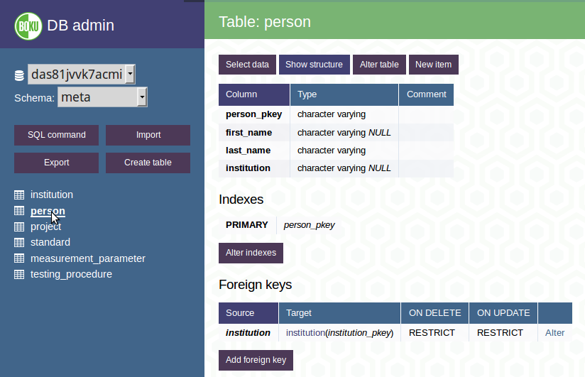
The database is organized in tables. Each table represents a certain entity with a number of arguments (the columns of the table). Each row is identified by a unique identifier, the so called primary key (primary keys in our database are, except for tables holding only one column, marked with the post-fix “_pkey“). The tables are connected by so called foreign keys, where a foreign key in one table references a primary key in another. Doing so, each information can be stored at only one place, the avoidance of redundancy ensures that your data keeps consistent.
5.1.2 Schemas
Besides other uses schemas can be used to organize database objects. For our purpose you can think of schemas containing tables such as you use directories in your file-system to organize files (You could make further use of schemas such as granting rights or avoid name conflicts, but this is not of big interest for our usage).
5.1.3 Queries
A query is a request for information from a database. You will be using a graphical user interface to interact with your data, but behind the scenes the front-end will “translate” your selections to the structured query language (SQL) and will send this SQL query to the database. Even tough you are interacting with an user interface, you will also always see the SQL code you send to the database below the controllers. The SQL code for an example query we go through further down this manual looks like this:

5.1.4 Views
Views are stored database queries. although views do not store data you can use them just as you would use tables. You can think of them as “virtual tables”, often showing data of two or more combined and/or subset tables.
5.2 Our database and how to use it
Our database uses all the above briefly explained concepts. It uses different schemas to organize the database objects:
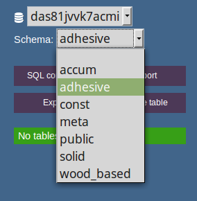
There are 4 schemas with actual data of major interest in the database:
- meta: holds all tables with metadata, such as testing procedures, projects, persons, institutions etc.
- solid: holds a table with the measurements for solid wood and various sub-types of it. The next section explains what a sub-type is.
- wood_based: holds a table with the measurements for wood based materials and various sub-types of it. The next section explains what a sub-type is.
- adhesive: holds a table with the measurements for adhesives and various sub-types of it. The next section explains what a sub-type is.
Two schemas hold tables containing only one column each, to restrict allowed values in other tables by using a foreign key constraint (resp. “lookup” allowed values):
- const: These tables contain “constant” values. These tables are very unlikely to change as they represent e.g. the naming convention for the measurement direction, allowed file-types etc. That said, the only use for this schema for any user is to look up allowed values. The column name in this one-column tables has no postfix as its obvious that it is the primary key.
- accum: Similar to “const”, but for “accumulating variables”. These tables are very likely to grow bigger as more extraction solvents are used, more pretreatments tried etc. The column name in this one-column tables has no postfix as its obvious that it is the primary key.
As explained above, views are stored queries combining or subsetting tables to create “virtual” ones. These views can be found in:
public: stores all views dedicated to the end-user. These are what you see when connecting through the easy approach
statistic: stores all views with calculated statistics.
summary: holds views counting measurements to provide some basic summary about the database entries.
In future there will likely follow additional schemas as they provide a good way to give limited database access to different user groups (e.g. external project partners) or to store custom views and tables related to different projects.
5.2.1 Selecting a schema
You can select the schema in the drop-down menu at the left panel
5.2.2 Open a table
To select a table click on the table name on the left panel or at the table summary on the body of the page. After doing so you see the structure of the table, the column names, their data types, the primary key of the table as well as foreign keys (the references to other tables - as explained above)
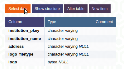
5.2.3 Get the data
If you’re not only interested in the structure of the table but also want to browse the data, click on Select data
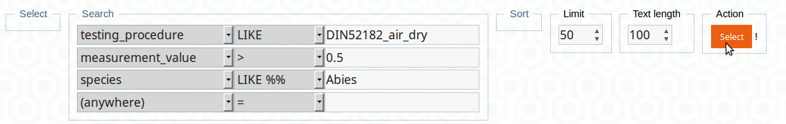
5.2.4 Filtering a data set
The DB Admin front-end is much more powerful when filtering data than the front end described earlier in this manual. You also click on Search and then you select a column, an operator and enter a value.
You can choose from many more operators here:
| operator | explanation |
|---|---|
| = | equal |
| < | less than |
| > | greater than |
| <= | less than or equal to |
| => | greater than or equal to |
| != | not equal |
| ~ | Matches regular expression, case sensitive |
| !~ | Does not match regular expression, case sensitive |
| LIKE | simple SQL pattern matching, case sensitive |
| LIKE %% | partial simple SQL pattern matching, case sensitive |
| ILIKE | simple SQL pattern matching, case insensitive |
| ILIKE %% | partial simple SQL pattern matching, case insensitive |
| IN | in set |
| IS NULL | is null |
| NOT LIKE | negation of LIKE |
| NOT IN | negation of IN |
| IS NOT NULL | is not null |
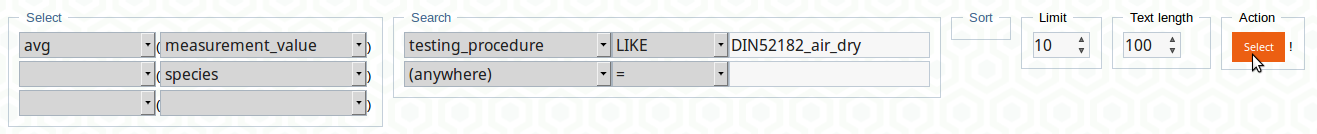
Using these operators the example below subsets all records with the testing procedure “DIN52182_air_dry” with measurement values greater than 0.5 and species partial but case sensitively matching “Abies” (like e.g. Abies alba, but could be others as well!):
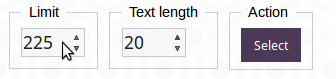
5.2.5 Show more results
You probably recognized that you only see a certain amount of rows on one page. In databases there is potentially much more information stored than would fit into the available memory of your computer (or the server where the front-end runs on). Therefore you can limit the shown information to a certain number of rows using “Limit”. Press the “Select” button after changing this value to update your query.
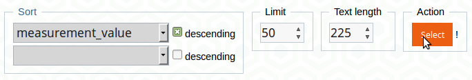
5.2.6 Sort the table
You can easily sort the table ascending or descending by clicking on the particular column name or selecting the intended column after clicking on Sort and eventually choosing descending.
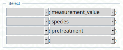
5.2.7 Select columns
Tables with a lot of columns are often difficult to overlook and therefore also difficult to understand. You can select certain columns of interest by using “Select” by just choosing column names in the drop-down menus surrounded by brackets.
5.2.8 Aggregate functions
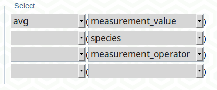
You can perform basic calculations within the database by using aggregate functions. To, for example, calculate the average value of measurement_value by species you simply choose the aggregate function and in brackets beneath you specify the column you want to apply this function to. Then in brackets below choose the grouping variable (species in out example) and press the Select button.
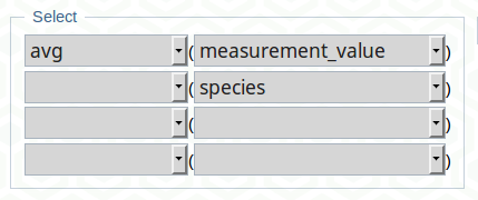
If you would be rather interested in the overall average, just use the first line, without selecting a grouping variable to get a single value as a result. But also more than one grouping variable is possible. You could, for example, calculate the average value per species and measurement_operator as easy as this:
5.2.9 Combination of aggregate functions, select, search and limit
In practice you will often combine all the methods shown above. You can, for example, calculate the average of the measurement_value measured according to “DIN52182_air_dry” by species, just showing ten lines like:
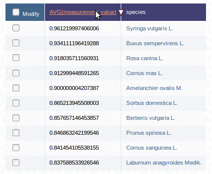
You can then press an the header of AVG(measurement_value) to see the ten lowest values (sort ascending) or press a second time to see the ten highest values (sort descending):
You can watch the SQL query change when you press the headers. The final query should look like this:
5.2.10 Download data to use it outside the database
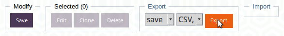
Once you are happy with your query, you probably want to download the data to use it outside the database. It works the same as described in the easy approach, click on Export after choosing an output format:
- TSV for tabstopp separated value
- CSV, for comma separated value using a comma to separate the values and a dot as decimal point
- CSV; for comma separated value (German version) using a semicolon to separate the values and a comma as decimal separator
5.2.11 Editing data
In case you find typos or error in the data and have sufficient rights to make changes you can do so by clicking on edit just left of the respective row, change the values, just as you would add a new entry and click Save.
5.2.12 Subtypes
It’s probably easiest to explain the concept of supertypes/subtypes resp. inheritance with the example of a webshop-database: Imagine you have a table holding data about the products sold by this webshop. The attributes represented by the table’s columns are e.g. the products price, package dimensions etc. But there are likely some attributes for certain products which are of no interest for other products. A book can, for example, have a number of pages whereas for a movie the duration can be of interest. Both remain products with the common attributes price and dimension.
A subtype (e.g. books) can therefore have additional attributes, while holding all attributes of the (“inherited”) supertype (products).
In our database for example the measurement table in the schema solid can hold some wood properties needing more attributes. These wood properties are represented by another table in the same schema with the prefix “stm_” (for subtype measurement) followed by the respective parameter (e.g. subtype stm_static_friction having two additional attributes “normal force” and “contact material”, not of interest for the other parameters).
When you add a new item to a subtype you will also have the entry available in the supertype (That saying, if you enter data to stm_static_friction, the entry also appears in the table measurement).
5.2.13 write your own SQL query
It is very likely that some needs are not addressed by the GUI functionality or by the provided views. In that case, or in case you just want to dig deeper into working with SQL databases, you can send any SQL query.
A good start is to take a look at the SQL strings when you build a query using the graphical tools. You can modify your query by clicking onto Edit at the right end of the string.
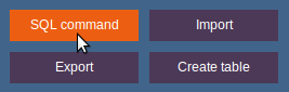
You can also write a SQL query from scratch, just click onto SQL command to do so:
Good resources to start with SQL are the PostgreSQL Documentation, the PostgreSQL Exercises and books related to SQL provided in the online library of the University of Natural Resources and Life Sciences, Vienna.
5.3 Additional information
5.3.1 is_valid
There is a column named is_valid appearing in all tables containing measurements. All uploaded data should be valid and therefore marked as TRUE in this respective column. However, it is possible that an erroneous dataset is appearing later - database administrators have the possibility to flag the row by setting the value to false. In case you stumble across a suspicious entry, please don’t set this value to FALSE autonomously, but rather contact a database admin to take a closer look at the entry.
5.3.2 User rights
Different users have variing rights on the database, dependent on what group the user has been assigned to. The following groups exist:
- admin: the admins are allowed to do anything with the database (even deleting database objects)
- data_admin: are allowed to connect to the database, select data, update (=replace) data, insert data as well as delete rows
- data_insert: are allowed to connect to the database, select data, insert data
- read_only: are allowed to connect to the database, select data